
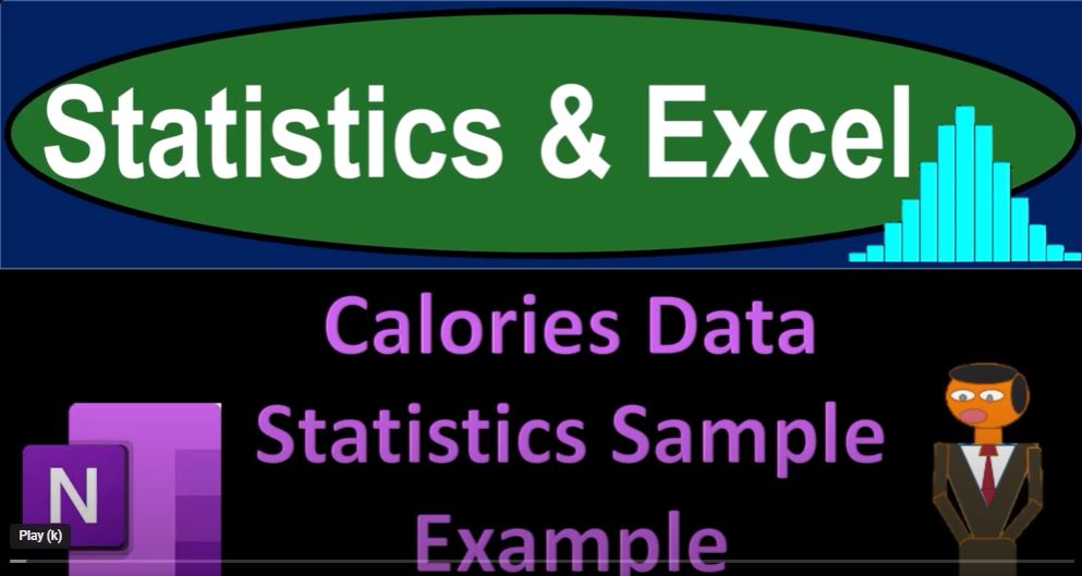
In the world of data analysis and statistics, Excel is a powerful tool that can help you gain insights from your data. In this blog post, we’ll dive into the exciting world of statistics and Excel, using a real-world example of calorie data. We’ll explore how to analyze the data, work with samples, and create meaningful visualizations to better understand the data.
The Dataset:
Our journey begins with a dataset containing information about calorie counts. The dataset includes dates and corresponding calorie counts. This data serves as an excellent example for our statistical analysis using Excel.
The Population vs. Sample:
Before we begin, it’s essential to understand the distinction between the entire dataset (the population) and the samples we’ll be working with. The goal is to use statistical analysis to draw conclusions about the entire population based on sample data. This approach mirrors what statisticians do in real-life scenarios.
Descriptive Statistics:
The first step is to calculate some basic descriptive statistics for the entire dataset. We’ll use Excel to compute the mean (average), median, maximum, and minimum calorie counts. These statistics provide insights into the central tendency and the range of our data.
Creating Histograms:
Histograms are powerful tools for visualizing data distribution. We’ll create a histogram in Excel to display the distribution of calorie counts in our dataset. The histogram will help us understand how the data is distributed across various calorie ranges, shedding light on patterns within the data.
Sampling:
To draw conclusions about the population, we need to work with samples. We’ll use Excel’s random number generator to shuffle the data and create multiple random samples. The randomness ensures that our samples are representative of the population.
Analyzing Sample Averages:
We will calculate the average calorie count for each of the 75 random samples, each containing 20 data points. This will help us assess how well the samples represent the entire population. We will compare the average of our samples to the average of the entire dataset to identify variations and trends.
Histograms of Sample Averages:
Next, we’ll create histograms of the average calorie counts for our 75 samples. These histograms will allow us to visualize how the sample averages are distributed and compare them to the overall dataset’s average. The varying shapes of these histograms demonstrate the impact of different sample sizes on our analysis.
Conclusions and Implications:
In conclusion, our exploration of statistics and Excel has revealed the power of data analysis and visualization. By working with different sample sizes, we gain a better understanding of how samples and sample sizes can affect statistical analysis. This exercise not only enhances our statistical knowledge but also improves our skills in using Excel for real-world data analysis.
By practicing with Excel, you can better prepare for future data analysis tasks and make more informed decisions. This example demonstrates the practical application of statistics and how you can leverage Excel to gain insights from your data.
So, are you ready to embark on your statistical journey with Excel? Start exploring your data, conducting analyses, and creating visualizations to unveil the hidden stories within your datasets. Excel is your trusted companion in this exciting adventure!