
In this presentation, we will delve into the intricacies of the Last-In, First-Out (LIFO) inventory system, focusing on the periodic inventory method rather than the perpetual one. Throughout our discussion, we will draw comparisons between LIFO and other systems, such as First-In, First-Out (FIFO) and the average cost method. Additionally, we will explore the differences between the periodic and perpetual inventory systems. To illustrate these concepts, we will use a comprehensive worksheet, which will prove invaluable for addressing various inventory flow assumption problems.
The Inventory Worksheet:
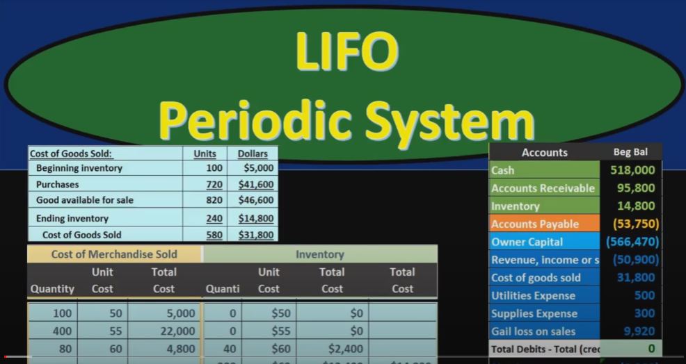
The worksheet we will be working with is divided into three main sections: Purchases, Cost of Merchandise Sold, and Ending Inventory. Each section is further divided into quantity, units, and total. This arrangement enables us to clearly differentiate between the purchases and the costs of goods sold, ultimately contributing to a more systematic inventory tracking process.
Getting Started:
Let’s begin with the opening transaction, the beginning inventory for March. We kick off the month with 100 units, each valued at $50, amounting to $5,000. It’s crucial to remember that the purpose of this worksheet is to support and substantiate the inventory information on the trial balance, ensuring that it aligns with what is presented on the balance sheet. We can think of this worksheet as the detailed backup for the inventory values on the financial statements.
Recording Purchases:
Our next transaction involves a purchase of 400 units at $55 each on March 5th. This purchase is straightforward, and its treatment remains consistent across different inventory methods. We will add the cost of this purchase to the overall inventory amount.
Here’s the journal entry for the purchase:
- Debit: Inventory (increases by $22,000)
- Credit: Accounts Payable (increases by $22,000)
Once posted, this purchase increases the inventory value on our worksheet to $27,000, ensuring that it matches the trial balance.
Handling Sales:
In a periodic system, we record only half of the sales transaction. The sale of 420 units at $85 each on March 9th is one such transaction. Here’s the journal entry for the sale:
- Debit: Accounts Receivable (increases by $35,700)
- Credit: Revenue (increases by $35,700)
This entry is common for both the periodic and perpetual inventory systems, as it captures the revenue generated. However, in a perpetual system, we would also record the decrease in inventory and the associated cost of goods sold. Under the periodic system, this cost of goods sold isn’t recorded until the end of the accounting period, in this case, the end of March.
Subsequent Purchases:
Continuing with our transactions, we make additional purchases during the month. On March 18th, we acquire 120 units at $60 each, and on March 25th, we purchase 200 units at $62 each. The rising prices reflect typical market conditions. These transactions, again, impact the total inventory value on the worksheet.
The journal entries for these purchases follow the same pattern:
- Debit: Inventory (increases)
- Credit: Accounts Payable (increases)
Once posted, these purchases are reflected in the worksheet, and the inventory value aligns with the trial balance.
Performing a Physical Inventory Count:
At the end of the month, we conduct a physical inventory count. In this step, we determine how many units remain on hand. This count helps us assess how much of the inventory we have sold during the month. In a periodic system, this adjustment isn’t recorded until month-end.
Calculating Cost of Goods Sold:
Now, we need to figure out the cost of goods sold for the entire month. This calculation is crucial for both the perpetual and periodic systems. The formula we use is:
Cost of Goods Sold = Beginning Inventory + Purchases – Ending Inventory
In our case, the beginning inventory was $5,000, and we made purchases throughout the month, resulting in $46,600 of goods available for sale. After our physical count, we discover that 240 units are still in inventory, leaving 580 units sold.
We use the Last-In, First-Out (LIFO) assumption to determine which units have been sold. Under LIFO, we assume that the most recently acquired units are the first to be sold. This affects the cost of goods sold calculation.
In units:
- We sold 200 units at $62 each
- We sold 120 units at $60 each
- We sold 260 units at $55 each
- The remaining 100 units were not sold
The total cost of goods sold for the entire month is the sum of these amounts, resulting in an accurate cost of goods sold for March.
Adjusting Entries:
The final step in the periodic system is to make the adjusting entries. These entries are performed to account for the cost of goods sold and the reduction in inventory, which were not recorded at the point of sale.
The adjusting entries are as follows:
- Debit: Cost of Goods Sold
- Credit: Inventory
These entries reflect the cost of goods sold for March and reduce the ending inventory. Once these entries are posted, the worksheet shows the updated ending inventory value, which matches the trial balance. The balance of inventory now accurately reflects the cost of goods remaining on hand.
Conclusion:
In summary, the Last-In, First-Out (LIFO) inventory system, when applied in the periodic inventory method, necessitates periodic physical counts and adjusting entries at the end of an accounting period. It assumes that the most recently acquired inventory is the first to be sold, impacting the calculation of cost of goods sold. The inventory worksheet serves as a valuable tool for keeping track of these transactions and ensuring that the financial statements accurately represent the company’s financial position. Understanding and correctly implementing the LIFO inventory system is essential for businesses aiming to manage their inventory and financial reporting effectively.