
In this presentation we will discuss first in first out or FIFO using a periodic system as compared to a perpetual system. As we go through this, we want to keep that in mind all the time that been that we are using first in first out as opposed to some other systems lastin first out, for example, or average cost, and we’re doing so using a periodic system rather than a perpetual system. Best way to demonstrate is with examples. So we’ll go through an example problem. We’re going to be using this worksheet for our example problem. It looks like an extended worksheet or large worksheet, but it really is the best worksheet to go through in order to figure out all the components of problems that deal with these cost flow assumptions, including a first in first out lastin first out, or an average method, and using a periodic or perpetual for any of them.
00:56
If we could set up the worksheet that would look something like this, then We can set up the same type of format for any of those types of problems. And you can see if you mix and match the fact that we can have a perpetual or periodic system for those three methods FIFO, LIFO, and average, there’s actually a lot of problems that could be asked that are slightly different in terms of methods with regard to inventory cost flow assumptions. So the format of the worksheet is going to be three columns or three separate sections purchases, cost of merchandise sold and inventory. When considering the periodic system as proposed as opposed to the perpetual system. We don’t really need this middle section until the end until we finally do the final calculation, which is where most problems will probably be focused because that’s where the adjustment will happen.
01:45
Until that happens throughout the time period. We’re just going to be recording the purchases, and then we’re going to record the what is still there, including what was there before plus the purchases to see what would be in Indian inventory. And each of these sections, we have at least three components. And those components will be the quantity, the unit cost and the total cost. And we’ll have to do a conversion each time because clearly inventory some type of units, some types of quantity that we will then have to apply some type of dollar to in order to get them on the financial statements. In other words, we cannot put quantity on the financial statements, we have to put dollars on the financial statements and therefore convert the quantity of the inventory we have to dollars in some way, we’ll have the same thing for the cost of merchandise sold.
02:33
Once again this column not being used so much so frequently, as in a perpetual system in the system, we will be using a periodic system. And then we’ve got the ending inventory, which will have once again the quantity the unit and the total cost. If we have this setup, then this will be workable for any kind of inventory flow a problem generally and we can put the information into this system and fix out not just the cost of goods sold, or not just the ending inventory, but both components of them. So going through this problem, we’re going to say that we have the beginning inventory first. So this is gonna just be the given of most problems. This is where we start this where we’re at at the beginning of the month or the end of last month. And that’s where we will start our worksheet. So we had 100 units, we’re just going to put them in the Indian inventory, they’re not being purchased at this time, they were purchased sometime before this month, sometime before March. And then we’re gonna have the unit cost, we’re going to say the first inventory we had cost $50. And if we multiply 100 times 250, we get the 5000.
03:40
The 5000, then is what would be on the income statement, I mean, on the balance sheet, or the trial balance, and this is the amount that will be on the financial statements. I’m going to repeat that over here and pull it out to the left side because later on we will have multiple rows and we’ll want to sum up to see what will actually be The total that will be reported on the financials. So here’s our beginning balance. If we were to compare that to the financials or in our case, the trial balance in order, assets, liabilities, equity, income and expenses to zero representing that we are in balance, the debits being in positive numbers, the credits being bracketed, and therefore debits minus the credits equals that zero net income net here is a loss at this point where we have no revenue, just expenses, the 500, the 309,009 20, being that 10,007 20 We, of course, are concentrating here on the inventory, which now matches our worksheet. So you can see that this worksheet, this is just the last column of the worksheet is tying out to what we have on the trial balance that will be consistently what will happen.

04:52
And you can compare this to if we had the accounts receivable here, for example, it has a supporting ledger. All of these accounts have supporting Ledger’s including inventory of the general ledger by date. But remember that an account like accounts receivable wants a supporting ledger, not by date, but also by customer who do we who owes us money? And inventory is going to be a similar way we want to see supporting data, not just by date, but buy inventory item, what what how many units do we have, and what’s the cost of those units. Now we’re going to go to the next thing that happens, which is going to say we purchased on 354 hundred units at 55. Notice that the last units we purchased were at 50. We have a rising prices. That’s the problem. And that’s the problem because prices don’t stay the same. Even though we’re buying the same units. These are the same widgets, whatever we’re selling, the inventory we’re imagining here, all the same, but the price is going up due to If nothing else, inflation.
05:51
Now it is possible for prices to go down but you want to really think of going up as the norm and then going down being pretty much the opposite. When we think of The effect on the financial statements. If we know what is happening if we know the difference in the comparison, as prices increase, we can easily just reverse them for the condition where prices decrease. So we’re going to say then on our worksheet on March 5 is going to be the next item here, we will say that we have 400 units, it’s going to start off in the purchases here, we’re going to list the purchases separate so we can see all the purchases in its own section. Then we’re going to add the purchases over here to the Indian inventory to what we already have in the beginning, and get to our ending inventory number. So we got 400 units and the purchases, they cost $55 400 times 55 is the 22,000. Now we’re going to pull that information over here to the ending inventory. In order to do so we will first bring down this number, this is going to be our first layer.
06:53
We want to have it in the same date range because that’ll just make things easier to look through. So we’re just going to pull that whole thing down, we just copied this whole thing down here, just so it’s all under the same date range, we’re not copying the 5000. Because that’s going to sum up the full layers for any date range here for March 1, here for March 5, it’s not going to just be that it’s going to be that plus this 22, which we will now put in the ending inventory as well. So we’re going to move that over and copy it over here. So there is some repetition here. Of course, we have to copy this over and copy this over, but by so doing that, we can have everything on this dateline. And we can show the purchases in a separate column so that we can clearly see the purchases column and the cost of goods sold column. Then we’re just going to add up these these two outer numbers under this date line. So remember, we only care now about everything under this green line. That’s all that matters.
07:49
At this point in time, we got the 5000 plus to 22,000 means we’ve got 27,000. So we have two layers of inventory now under first in first out Got the 100 units at 50. We’ve got the 400 units at 55. Under first in first out, we would assume that we sell the 100 units first, although remember, that’s just an assumption the people purchasing could purchase any unit they want. Because possibly we haven’t even labeled them to be able to distinguish which is which we’re just assuming that the the first units were going to sell first. Then if we did the journal entry behind this, we would say Okay, now we’re going to record the journal entry for this purchase here that we made this purchase here and see what happens in terms of transactions. It’s important to tie this worksheet out to the financial statements here. So we’re going to say okay, here’s the inventory, it has a debit balance of 5000.
08:46
We bought 22,000 more of inventory. Note, this is not an estimate, this is going to be the same whether we use FIFO LIFO, average specific identification, perpetual periodic system under any of those methods. Always the same. Not an estimate, it went up for whatever it’s going to go up for, we’re going to pay 22,000. Because it has a debit, we’ll do the same thing to it another debit. So we’ll debit inventory, we’re going to assume we didn’t pay cash but purchased it on account and therefore cash will not be decreasing the good things not going down the bad things going up, we owe accounts payable. So accounts payable has a credit balance, we’re going to make it go up doing the same thing to it another credit. So if we post this and if we post this to our worksheet, we have the 5000 plus the 22,000, giving us 27,000. Then we post this accounts payable to our worksheet, we’ve got the 12,001 50 plus the 22,000 meaning we owe now 34,150. So if we were to see that all together, then here’s all the numbers filled out. This is our beginning balance worksheet.
09:53
Here’s our adjustment that we made. Here’s where we end up here’s the ending balance after that adjustment, we can see that the 20s 7000 here matches what is on our worksheet. So it supports the worksheet supports what is on the financial statements, what is on our trial balance. Note, there’s no effect on net income. Even though we purchased inventory, we’re not going to expense inventory at the point of purchase, we will expense it when we consume it in order to help us generate revenue in the form of cost of goods sold. However, we won’t make that adjustment under a periodic system until the end of the period, the end of the month, the end of March in this case, next item, we’re going to say that there was a sale of 420 units at $85. Now note what we’re not showing here, here, we’re not showing the worksheet for the cost worksheet, because under a periodic system, we only record the sales component of it, we’re not going to record the related cost component until the end of the period until we do a physical count.
10:55
This is really the difference between the two methods in terms of the transactions As we go through the period, so in terms of a periodic system, we will record the journal entry, but nothing will be recorded to the inventory accounts nothing will be reported to the new accounts. When we go from a service company to a merchandising company, those accounts have inventory and cost of goods sold. What we will record is the first half of the transaction that we typically think of when we make a sale of inventory, the transaction that would be the same in many respects, in all respects pretty much of a service company if they did work and got revenue. So if a service company did work and got revenue, they would say that they did if we didn’t get cash, we did it on account, we got accounts receivable, accounts receivable would increase. So accounts receivable is going up by 35 seven, which is 420 units times $85. And then the other side would go to revenue revenue is a credit balance account.

11:55
We’re going to make it go up by doing the same thing, another credit so we would credit Then revenue. So there’s going to be our transaction debit in accounts receivable credit in revenue. Note as well that this $85 has nothing to do with our worksheet in terms of the cost, it only has to do with the sales price, we may use the cost to generate to figure out what the sales price will be. But the cost is what we are dealing with mainly in this problem, the sales price is going to be something different from the cost and we’re gonna have to figure out what the sales price is. That’s not what we’re tracking in our worksheet. The journal entry we are not doing is this half meaning inventory is not going down and cost of goods sold is not being recorded. Why? Because we’re using a periodic system.
12:43
Why would we use a periodic system? Possibly because our system is not sophisticated enough in order to do a perpetual system. In other words, I know we know even if we have like a clerk working at the front of the store that what the sales price will be Because it’ll be on the sticker price. But we may not know what the cost is, especially if we have multiple types of inventory. And therefore, it will be easier to make the sales transactions what we’re concentrating on when we’re trying to generate money, if we just record this half of it at the sale, and then record this half at the end of the time period, If however, we had a more sophisticated system, such as a scanner that could report this information as it happens real time without us even needing to know about it or deal with it, then we could we can use a perpetual system which would be better for the accounting purposes as we go, so we’re going to report or record this side. Now here’s accounts receivable here. Here’s our accounts receivable up here.
13:45
We would then be increasing accounts receivable with a debit, bringing it up to 80,600. Then we have the sales 35,007 credit, nothing’s in sales over here. We’re going to increase it 35,700 to 35,000. 700 if we see the full accounts, then here’s where we started. Here’s our journal entries. Here’s where we ended up, we can see that of course, the accounts receivable went up, and revenue went up, bringing net income up net income calculated as this revenue 35 700 minus these expenses 500 300 909,009 20 given us revenue, not a loss revenue, these are these accounts right here of 27,980. Now, note this amount is totally off, because we do not record at this point Cost of Goods Sold Cost of Goods Sold has not been recorded, we only recorded the increase in revenue. Therefore, our net income under a periodic system is very not correct until the end of the period. So we just have to recognize that as we go and not make decisions on this number because it’s not accurate until we record the cost of goods sold, as well as the increase in inventory which also is not correct.
15:00
At this point in time, because we obviously gave up some inventory to generate this revenue, and have not yet recorded under the periodic system, we will record it at the end of the period, the end of the month, the end of March in this case. Next transaction, we’re going to say on 318, we purchased 120 units at $60 per unit. So here’s where we started off last time, we’re going to continue right here on March 18, we’re going to say there’s another purchase. So it’s going to look like a similar transaction, we’re going to be in the purchasing side here, we’re going to say we got 120 units, they cost $60. Note the rising prices from 50 to 55 to 60. If we multiply the 120 times the 60, we get these 7200. We’re then going to pull this information over to the Indian inventory item to see what is still there. Now, at the end of the time period. We’re going to pull down this information what we already had. So these two columns or rows, we’re going to pull those down, that inventory is still there.

16:04
And then we’re going to add to it this inventory item. So now we have three layers of inventory, we’ve got 100 units at 50, we got 400 units at 55. We got 120 units at 60. They’re all the same widgets, they’re all the same thing. They have right they have different prices, Andre first in first out, we assume we sell this one first. Note, we’ve already made a sale and we may have made more than one sale. I just recorded one as an example. But we didn’t reduce it yet. We will reduce it at the end of the time period when we do the physical count and note that because of that, because the layers could be different throughout the time period. That means that a perpetual system and a periodic system even after the end of the month after the adjustment has been recorded, could differ even using the same flow assumptions such as first in first out.
16:54
So if we use a perpetual system and a periodic system, under first in, first out It is possible for us and but not necessarily the case that we end up with a different numbers at the end of the time period even after the recording of the adjustment. So then we’re going to add these up, we’re going to say okay, the 5000 plus the 22,000, plus the 7002. That gives us the 34,200. This is what should be on our financial, this is what should be on our trial trial balance. We’re now going to record the purchase again, and see that this number which should be what we end up with, with inventory, note that these purchases once again, don’t change under any method first in first out last in first out, average identification, perpetual periodic video will be the same as will the journal entry that we will record now. So here’s the journal entry. Here’s our new transaction that we had here, the 7200 that we purchased, it is what it is doesn’t change under either method.
17:51
We’re going to say that inventory is what we purchased, it has a debit balance, and we’re going to make it to go up by doing the same thing to it. Another debit. So we will debit The inventory. The second component will be the way we paid for it not with cash. In this case, we bought it on account. So we have accounts payable as a liability, it’s going to go up by doing the same thing to it another credit. So if we post this out, then we’re going to say here’s the inventory started at 27,000, it’s going to go up by 7200 to a total of 34,200. Here we have the accounts payable started at 34,150 is going to go up by 7200 to 41,350. If we see all those accounts, then here’s what we have. And obviously inventory went up to 34,200. That’s what we have on our worksheet our worksheets supporting that number on our trial balance. The accounts payable is is here and no effect on the net income. No effect down here. Even though we bought inventory.
18:56
We didn’t expense the inventory at the top purchase. We put it on books as an asset, we will expensive when we consume it to generate revenue in the form of cost of goods sold. However, we won’t record that cost of goods sold under a periodic system till the end of the period, the end of the month, the end of March in this case, next transaction 325 purchase 200 units at $62 per unit. So, note we’re only recording the purchases here in this worksheet, and then we might have more sales happening but I’m not going to record all the sales, because that’s not what’s going to be recorded. In this worksheet, we’re going to figure out the cost of goods sold related to the sales at the end of the time period with a physical count. So it’s going to be another purchase another familiar transaction on March 25. We purchased 200 units $62 note the rising price is 55 to 60 to 62. It started at 50 at the beginning, and that gives us 12,400 we have the layers here before the one Hundred, the 400 to 128 5055 and 60, we pull those down.
20:04
So they’re all under the same dateline. So as of March 25, I only want to be working with stuff that’s under this green line. So that’s why we have to pull all this down. And then we’ll pull this over, adding one more row. So now we have 100 units at $50 400 units at $55 120 units at $60 and 200 units at $62 for a total of 5000 plus 22,000 plus 7200 plus 12,400 or 46,200. This then should be what is on our financial statement after we record this transaction, which doesn’t change under either method, FIFO LIFO, average periodic perpetual, it is what it is. Here’s the journal entry. We’re going to record this transaction this 12,000 that we 400 that we purchase. It’s going to be inventory increase in inventory has a debit balance 34,200 We need to make it go up doing the same thing to it debiting it, then we’re going to increase not the cash but accounts payable accounts payable as a credit balance, we do the same thing to it another credit. If we post this, then we’re going to say that this is the inventory 34,200, we will increase it by the 12,004.
20:04
And then it’ll go up to 46,600 matching our worksheet, then the accounts payable is here, we’re going to post that to this 41,003 50 increase in it by 12,400 to 53,750. The main point here being that the inventory is matching the 46 600 matching and supported by our worksheets here. Next thing we’re going to do, we’re going to say at the end of the period now and we had Indian inventory that we will then count. Now this is going to be the key component to the periodic system. What we have not done is record the middle column. We haven’t recorded the cost of goods sold not showing In the cost of goods sold column here to save some space, we only have the purchases and the inventory, we will be working on the cost of goods sold to figure out now, what we did sell how much of the inventory we sold How? First we’re going to figure out how many units we have left with a physical count. So we’ll take a physical count, we’ll say how many units we got left, we’ve got 240 units, then we typically look at this in terms of the cost of goods sold calculation.
20:04
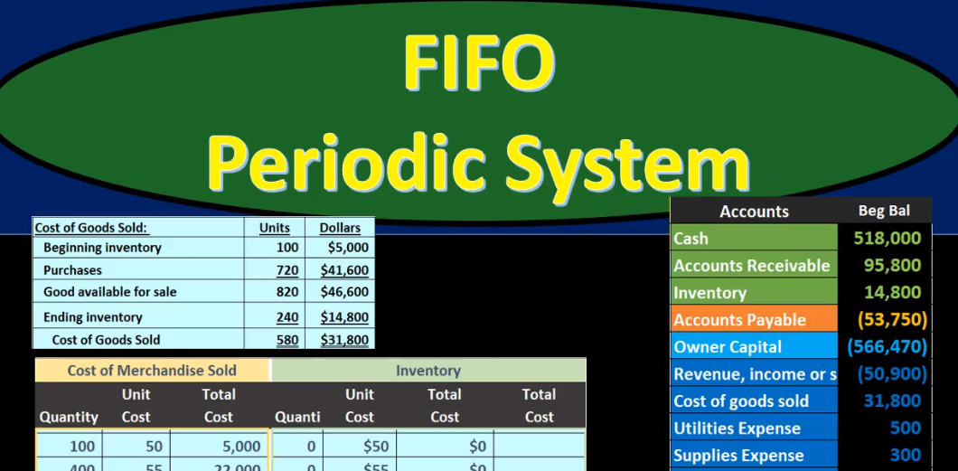
Note that this 240 units is in units and our numbers here are in dollars. So the fact that there’s a conversion problem, and more complicated by the fact that the costs are not all the same, even though we have the same amount or kind of inventory means that we have to do some type of conversion, it’s a little bit more complex. We can do this cost of goods sold calculation in terms of both units and dollars. Cost of Goods Sold calculation must be memorized. It’s it’s kind of an essential component and it goes on This, we got the beginning inventory where we started at the beginning of the time period, we’re going to say purchases. And then typically we have a sub category subcategory being our goods available for sale. So whatever we had at the beginning, plus whatever we purchased through the entire month, is what we could have sold during the time period. It does not mean that we had that amount at any point in time during the time period, it means that that’s how much went through the the accounting department or our warehouse during that time period.

23:32
And therefore it could have been sold at some point through the time we’re in our case, the month of March, then we’re going to subtract from that the ending inventory, the amount we counted the amount we counted, and that will give us the cost of goods sold. So this will be the typical calculation you just got to kind of memorize this. Note that this cost of goods sold or goods available for sale is a subcategory. You could just have beginning inventory plus purchases minus ending inventory. eliminate this sub category. But you want to know that subcategories name, because it will be named oftentimes in problems and in practice. So we’re going to do this first in units and then in dollars. So we’re going to say beginning inventory and units was this 100 units.
24:16
That’s what we started with purchases. That’s why it’s nice to have the purchases column set out here was 400 plus 120 plus 200, we could just add those up the quantity the units given us 720, meaning that in units we could have sold 820. Now that again, doesn’t mean we had 820. At any point in time during the time period we could have been selling throughout this entire time period. But that’s how much went through the warehouse through this time period and therefore was available for sale and could have we could have sold at that time. Then we’re going to do the physical count the inventory count 240. That’s what we counted the inventory to be if this is what we could have sold. If this is What went through the warehouse at any given time, and we only have this in the warehouse now as of the end of the month, then we can subtract the 820 available minus what we currently have.
25:11
And assume we have cost of goods sold of 580. Note there is an assumption there because it assumes that we sold these units as opposed to last them have been stolen broke them or something like that. And, and that’s part of the problems with a periodic system in that in a perpetual system, we can have an easier calculation to kind of figure out how much might have been done to shrinkage, some kind of loss or theft, as opposed to sales. But our hope is that most of this was sales and the port that was theft or loss or some other component is not significantly high and therefore will still record the cost of goods sold as the cost of goods sold. In other words, it would be in material to decision making. Now we’re going to do the same thing in terms of dollars. Same Cost of Goods Sold calculation beginning inventory was 5000. Then we had purchases, which was this 22 plus two, seven plus 212. And it purchases side purchases column, giving us 41,600. If this is what we had in dollars at the beginning, this is what we purchased.
26:18
No estimate here it is what it is, that’s what we purchased for, then we’re going to have 46,600. Notice that again, this item here is going to be the same under any method, it’s going to be first in first out last In First Out perpetual period, it purchases what we purchased. So we got the 46,600. Now we’ve got the ending inventory. That’s where the problem is because we know the units, but I can’t just convert the units to dollars because we know that the units all cost different amounts, we have to use a cause that’s where the estimate is going to play in. So this is kind of where we have to stop until we go back to the worksheet and say, Okay, well, which units did we sell and how much did they cost? So we’re going to do that here. Remember, we had 100 units at $50 400 units at 55 120 units at 60 and 200 units at $62. Under a first in first out method, we assume we sold these units first.
27:15
Now note what we have here, this is our worksheet, we got the ending inventory and the cost of goods sold column. Now, this column that we haven’t used the entire time period, which we are now using, at the end of the time period, you could think of this problem a couple different ways. If you see it in multiple choice questions, they may only ask you for, for example, what is left in ending inventory? Or what is Cost of Goods Sold? But you really want to be able to set up the problem. So you can do both sides and be able to answer both. Both questions. That’s why a worksheet like this is good to be able to set up. So in other words, there’s 240 left here, so we could start at the ending inventory and try to figure out okay, well if I sold these ones first I’ve got the 200 left. And I could try to figure out how much of the 240 is left. Or we can say if we sold 240, then the unit I mean, if we have 240 left, then we sold 580.
28:13
And we could try to figure out, look at the same data and think of it from that side, we can say, Okay, if we sold 580, we sold this first, and then the second. So that’s how we’re going to do it here. We’re going to we’re going to use this 580 number, and try to figure out what we’ve been sold and record that in this cost of goods sold side. So in other words, if we sold 580 units, we’re using this number. Then we saw all of this hundred units at 50. We assume that that is gone. So this whole row has been wiped out here. So this row is basically gone. And then we sold 400 at 55. This rows basically gone. We sold all of those because we’re trying to get up to 580. And those are gone. And now we’re gonna say okay, how much do we have left here? Well, we got 580 is what we needed, minus 401 hundred or 500. That means we had 80 units that we must have sold at this layer. So we had 80 units that we sold at $60. And that’s going to give us 404,800. So this is going to be the layers we had of the 580 units, 580 units, we sold 5100 of them at $50 400 at 5580 at 60. That’s the assumption we have.

29:32
And that’s going to be our calculation if we add those up. Well, let’s first see what we have left now. Then if we see what we have left these remember we wiped these out. So those are gone. So this this row is now gone. This row is now gone, because 400 minus 400. So here’s the 400 minus the 400 is zero. The 100 minus the 100 is zero Then the 120. And minus two ad is going to say that we have 40 units left there. And that’s going to be that and then the 200. Of course, it’s just has not been touched, we have the 200 left. So what we have left then from these layers is these layers down here 40 units at $60 200 units at 62, giving us 2400 plus to 12,400 or 14,800. So we really need to be able to look at this from two perspectives what we sold what the cost of goods sold is and what we have left.
30:43
Now we have the ability to complete this we can say the the the ending inventory is going to be that 14,800 and then the 46,600 minus 14,800 will be the cost of goods sold 31,800 or 5000 plus 22 plus 4008 would give us that 31,800. If we go and we count and we make the journal entry, now the final journal entry that we have not been making this entire time period, this is the journal entry, we would be seen every time we make a sale under a perpetual system, the one we have not been seen, every time we make a sale under a periodic system, we haven’t even shown it all the time, just one time just to show the difference will be this. So this is the second half. Remember, when we make a sale, typically under a perpetual system, we break that journal entry into two components to think about it theoretically. One is the sales side, and the account receivable side, increase in accounts receivable, increasing revenue. That’s what we have seen what we have not seen.
31:46
What we did not do is the other side, every time we make a sale, decrease in the inventory for what we sold, and increasing the cost of goods sold. That’s what we’re going to do now for the entire time period for all sales that happened through the time period. through the month through March. So we’re going to say cost of goods sold is going to increase by Cost of Goods Sold 31,800. And the inventory then had been a debit balance is going to go down by all the inventory we gave up throughout the month 31,800. Once we post this, then this inventory we’ll be left with what we calculated ending inventory to be 14,800. So let’s post this we’re going to post the 31,800 cost of goods sold at zero increases 31,800 to 31,800. We’ll post the inventory then. So the inventory started at 46,600 increasing or decreasing with a credit of 31,800 to 14,800.

32:46
That then, of course matching our 14,800 here, and that’s going to be the key component here. If we see all the accounts put together we see the 14,800 our ending balance matches what we calculated here. We see now that our net income is affected dramatically, it’s going down. If the net income is 50,900 revenue minus all the expenses, this expense Cost of Goods Sold huge expense has just increased bringing net income way down from 40,000. net income down by 31. Eight to this 8003 80. This is still income, it’s not a loss. But until we record this huge component, this huge expense Cost of Goods Sold big number, then under a periodic system, our net income is drastically wrong until that adjustment happens at the time period. So we just need to recognize that of course, if we see our calculations, then we know that the cost of goods sold calculation, we can tie it out to the worksheet and tie it out to our numbers on the trial balance. It’s going to be the ending. This is our ending trial balance now, so we’ve got the cost of goods sold is here would match the 5000 plus the 22 plus the 4008. Same number here and of course it’s the same number on our trial balance. We can see that the ending inventory is 14,800 here also 14,800 on our worksheet and 14,800 on the trial balance.