
In this presentation we will discuss the lastin first out inventory system on a periodic basis rather than a perpetual basis. As we go through this process, we want to always be comparing those to one, the LIFO or lastin first out system to other systems such as first in first out and average, as well as comparing the perpetual system to the periodic system. We’re going to go through this by looking at a problem the problem going into a worksheet such as this, I do recommend learning this worksheet. This worksheet should look repetitive if you seen the first in first out presentation as well as presentations for the perpetual system.
00:42
That’s because this worksheet can be used in order to work most of the flow assumption problems. And there’s a lot of them if you think about the combinations we can have, including the lastin first out method we will be working here or the first in first out method and the average method. Both those can be done either on a perpetual or periodic system. So there’s a lot of combinations we could have, but they could all fit into this type of worksheet. Note that problems could ask a comprehensive worksheet such as this or problems could ask for small components. If we learn the entire worksheet, however, we can fit that problem or that worksheet to all the problems related to this type of system inventory flow assumptions, that format would be three sections that would be purchases, and then the cost of merchandise sold and then the ending inventory.
01:35
Within those sections, we’re going to have the quantity, the units and the total for each, and that will be able to allow us to separate the purchases from the cost of goods sold and the ending inventory. When we’re working in a periodic system as we are now we won’t be working with this middle column until the very end, when we make the adjustments at the end of the time period recording that cost of goods sold and Related decrease in inventory. So the beginning transaction will be the beginning inventory. So we’re going to say that we start off at the beginning of the month, in this case, March. By the way, as well note that these formats for the periodic system will look very similar for the systems including first in first out, and the lastin. First out until we get to the end of the problem, but we do want to go through theirs and just put together this worksheet so that we can see how it’s formatted and compare and contrast these journal entries as we enter them. So we’re going to put in the beginning balance 100 units, and they’re at $50 100 times 50 is 5000. So that’s where we start.
02:42
That’s the beginning balance that we are starting with at the beginning of March. Note the conversion we have to do here one from units to the dollar amount to get the $5,000 that will be reported on the financial statements. We’re going to pull that 5000 over to the right because later on, we’ll have multiple letters And it’ll be easier to see if we pull this out to the right. This being the amount we would see on the financial statements. We have the trial balance here, here’s going to be our trial balance. It’s in order assets, liabilities, equity, income and expenses. We know we’re in balance because the debit balances are represented without brackets or positive numbers, credits with brackets are negative numbers. And if we were to add all of them up, they add up to zero. net income currently is a loss. There’s no revenue and we have these expenses 500 309,009 24 loss of 10,007 20 This is our ending inventory that the last component that we just pulled over from the worksheet. 5000 is what is in inventory that matches what is on our financial statements or trial balance here.
03:47
That’s our starting point. It’s important to remember that this worksheet is in essence, backing up supporting being the detail behind this inventory information on the trial. Back balance or balance sheet. If we go through the next transaction, we’re going to say that there’s a purchase of 400 units at $55. notes that the price is rising, they were $50. Now they’re $55. That’s going to be the normal scenario. So the normal process our prices rising, we want to consider factors as prices go up. And then kind of reverse what would happen if there was a decline in price. So we’re going to say on March 5, we bought 400 units, which will clearly go in the purchases section, and they cost $55, to give us a total of 22,000. Note that this would be the same under FIFO LIFO average, it would be the same under a perpetual or periodic in either system. This is not an estimate or assumption. We’re then going to pull that over to the Indian inventory and add it to what we already have.

04:50
We want to have everything However, under this line at this date line so that we don’t start getting confused as the worksheet grows. Therefore, we’re first going to pull this down. So we’re just going to say this is the same information we just pulled down here. And now we have 100 units at $50. And then we’re just going to pull this over to have the 400 units at 55. So we have a total of 500 units, 100 of them cost us $50 400 of them costs us $55. If we were to sell something at this point in time and record it, we would assume under lastin. First out, we sold the last ones, we purchased these 401st. However, we won’t do that until the end of the problem. When we counted under the periodic inventory system. We’re going to add these up to 5000 and the 22,000, giving us the 27,000. That then will be the amount on the balance sheet or the trial balance. If we then record this, we’re recording this purchase. There’s 22,000 remember, doesn’t change under whatever inventory method we use. We’re going to say that we bought inventory inventory has a debit balance.
05:58
We got more of it. So We’re going to do the same thing to it, another debit will debit the inventory and then we will credit something not cash cash isn’t going down, we’re crediting instead accounts payable, the liability has a credit balance, we’re increasing it by doing the same thing to it another credit. So there’s going to be our transaction if we post this then this inventory at 22 will be posted here the 5000 going up by the 22,000 to 27,000. This 22,000 for the accounts payable will be posted here to accounts payable, the 12,150 will go up by 22,000 to 34,000 to 150. That’s going to be our transaction. Note that this 27,000 now matches what is on our inventory worksheet. If we look at the totals here, we see that they’re back in balance. Of course, we’re back and balanced debits equal in the credits, and there is no effect on net income meaning nothing happened in the revenue or expense accounts.
06:59
All we did was Purchase inventory. inventory is not an expense when we purchase it. It’s an asset when we purchase it, purchase it, it will be expensed however, but not until we use it in order to help generate revenue not until it’s expensed in the form of cost of goods sold. Next transaction three nine sale of 420 units at $85. This is the only sales transaction we’re going to show here because under the periodic system, we would not be recording this to the worksheet, we’re only going to be recording the sales half, which is not located on our worksheet. We will post the journal entry just to show the journal entry. If it were a perpetual system, then we would be recording the second component and we would be recording it to our worksheet we would be decreasing in other words inventory at the point in time of sale and recording the related cost of goods sold. However, here we will not so you If we think about a sales journal entry, we typically under a perpetual system, which we are not using here, think of it as two types of journal entries or we can think of it that way. And it’s really helpful to when learning these two journal entries, or the sales transaction of inventory, one related to the same type of thing happening if we were a service company, eliminating inventory and related accounts, and the other having to do with inventory recording the decrease in inventory. If we think about the first half of the transaction, the half that we could eliminate inventory accounts be very similar to if we were a service company.
08:35
We’d say we made a sale on account we didn’t get cash, we got something else we got an IOU, accounts receivable, it has a debit balance of 40, it will have a debit balance, we need to make it go up because people owe us more money. We do the same thing to it another debit. And then the other side of it will go to revenue, whatever that revenue called service company might be fees earned. It might be income, revenue, or sales depending on the type of company All the same thing in terms of the type of account revenue, revenue has a credit balance, we increase it with a credit. So this will be the same under a periodic or perpetual system. Also note that we have the 420 times 85. To bring us to that amount, what will not be the same if we won’t have the second transaction here under the periodic system, we won’t record the cost of goods sold the expense related to this transaction or the inventory. Now, you might ask why, why wouldn’t we do that? It seems reasonable to do that we clearly had given up inventory and it should be going down. But it’s usually with regard to the sophistication of our system. If our system is not an electronic system, we want to focus more on the sales process. So especially if we have something like a clerk or something making the sales, they may know the sales price, but they may not know what the cost is and note the cost will be different.

09:57
The cost will not be this at $5 It’ll be what we paid for the inventory, what we’re tracking on the worksheet. And if we don’t have a sophisticated system, we might not know that at the point in time of sale or want to have to deal with that at the point in time of sale, we will deal with it periodically as we count the inventory at the end of the time period. Also note that this 35,700, dealing with this 85 times 420. Once again, this 85 is not something that we’re going to see in our worksheet at all. It might have something to do with the cost, we might have used the cost to derive the sales price, but it has nothing to do with our cost worksheet. If we were to post this out, then we’re going to say accounts receivables here accounts receivable there in this journal entry. It’s going from 44,900 up by 35,700 to 80,600. Then we’re going to post the income the revenue or the income the sales going from zero up by 35,700 to 35. Thousand 700. Here’s all the accounts if we note the effect here, we see that net income is going up substantially by the income here, it was at a loss, we have this revenue.
11:11
This is not a loss, this is revenue over expenses 35,000 minus the 500 miles 300 minus 9009 20 given us revenue, note that this net income number is substantially wrong. Because we haven’t recorded the cost of goods sold under the periodic system, it will be right at the end of the month, when we do the calculation of the physical count of in Indian inventory, recording the decrease in inventory and the related cost of goods sold. This 27,000 also wrong until we get to the end of the month, count the inventory, make the adjustment so we’re still at this 27,000 on the worksheet. Next transaction, we made another purchase 120 units $60. Note the rising prices 50 to 55 to 60. That’s the new You want to think about that as normal. And then if they reverse that, if you see the prices going down, you’ll just have to reverse some of the assumptions we make or some of the outcomes that will happen. So we’re going to say on March 18, we have 120 units in the purchases section, of course, and we are saying there’s $60 each, if we multiply 120 times 60, we get 7200. Once again, we want to take this information and put it below this line and have everything below this line.
12:30
To do that, we’re going to say everything at this date line. below this line is what we had before. 100 units at 5400 units at 55. We’re just going to bring those down to our new section here. And then we’re going to bring these items over. So now we’re going to add the new rows. So that’s what we have now we have 100 units at 50. We got 400 units at 55. We got 120 units at 60. If we were then to add these up, we would say that we have total inventory of 35 4200 in terms of dollars, we’re going to then record this purchase. And remember this purchase doesn’t change whether using FIFO or LIFO, average perpetual or periodic. If we then do the recording, we’re going to say that we got this 7200 purchase inventory is at 27,000.
13:19
We need to make it go up, we’ll do the same thing to a debit debiting inventory, the other side not to go into cash, we’re going to assume we didn’t pay cash but bought on account. Therefore the accounts payable credit will go up in the credit direction 7200 then we’re going to post this out. So here’s the inventory here. Here’s our inventory there it starting at 27,000 going up by 7200 to a total of 34,200. Then we have the accounts payable here it’s going to go to the accounts payable, they’re starting at 34,001 50 going up in the credit direction 7200 to 41,350. This Indian inventory that’s Where we’re focused, because that matches what we’re tracking the support of that number, that being the inventory worksheet, we look at all the numbers, here’s what we have. We note that there’s no effect on net income. net income isn’t affected because no income revenue or expense accounts are affected, we will expense the inventory but not at the time of purchase at the time we sell the inventory in order to generate revenue. We won’t do that on a periodic system, until we count the inventory at the end of the period, in this case, the end of the month, the month of February.
14:33
Next transaction another purchase. So we purchased 200 units at 62. Note we’re not recording all the sales here because the sales aren’t affecting this worksheet. And this is one thing we have to note when we work through these worksheets, we have to note that we’re zooming in on a particular thing and still have an idea of how it fits into the overall picture here. So the 200 is going here. And note if we were in a perpetual system, we would be recording the cost of goods sold here as we go. So now we’re going to say on March 25, we had 200 units $62. Note the rising prices 50 to 55 to 60 to 60 to 200 times 62 gives us 12,400. Now we’re going to bring everything below this line here. We want everything below this line on the ending inventory, very jagged line, more like some crazy curve. But here’s what we had before. 100 units at 5400 units at 55 128 60. We still have those, or we may not physically have those, but they’re still recorded on ours, our inventory sheet, we did make sales and have sold some of those, but we haven’t known which one yet.
15:44
We’ll do that at the end of the process. So we’re really calculating goods available for sale here. So here we have those here. Now we’re going to add the new layer. There’s the new layer. So now we got 100 units of 5400 units at 55 120 units at 6200. You 60 to 5000 plus 22,000 plus 7200 plus 12,400, giving us 46,600. So that 40,600 should be what should be on the financials or the trial balance. We’re going to record this to the trial balance. Remember that this amount the purchase is not an estimate doesn’t change, whether using FIFO LIFO, average, or perpetual or periodic. We’re going to record this purchase. Once again, journal entry should look familiar. We’re going to say that inventory has a debit balance, we bought more of it, it’s going to go up by doing the same thing, another debit. We didn’t pay cash instead, the bad things going up rather than the good thing going down. Accounts Payable liability increasing has a credit balance, we increase it doing the same thing a credit.
16:47
So there’s our journal entry. Here’s inventory. There’s inventory here. It starts at 34,200. It’s going to go up by 12,400 to 46,600. Here’s our accounts payable Here’s our accounts payable there, it’s starting at 41,003 50, it’s going to go up in the credit direction by toward 12,000 to 400, to 53,750, the concentration note here, inventory 46,600, supported now by our schedule, the 40,000 46,600. Next, we’re going to take a look at our ending inventory count. So we’re going to say that we counted the inventory to be 240. This is at the end of the time period month is over. Now, we’re going to do a physical count. And now we do that in order to help us decide on in a periodic system, how much of this available for sale inventory, how much of these layers of inventory or the 100 plus the 400 plus the 120, close to 200 units that we have right now? How much of those have we sold and kept? to do that? We typically look at a cost of goods sold calculation and mandatory calculation, one that we need to understand no matter what What system we are using, we can see it in terms of units, we can do the same calculation in terms of dollars.

18:05
Both are something that is necessary for us to know, the format will be beginning inventory. This is the generic format that we apply all the time, beginning inventory, plus purchases, that gives us the subtotal available for sale. That subtotal representing what we had available at any given time doesn’t mean we had that inventory at any point in time, but throughout the entire month, that’s how many widgets went through the warehouse. That’s how many widgets we could have sold, given the fact that we had them at some point during that time process. Then we’re going to subtract from that our count our ending inventory, which we would get from the physical count here, and if this is what we had available throughout the time period, and this is what we still have at the end of it. The difference between those two will be our cost of goods sold.
18:54
So it’s beginning inventory plus purchases gives us goods available for sale, minus ending in ending Inventory gives us cost of goods sold. Note that we this is just a subtotal. You could eliminate this if you just want a formula for algebraic reasons, because questions could ask this in any format, they could, you know, give you all the numbers except one of these, and you just write out this same algebraic equation. In order to solve it. What you don’t want to do is to figure out and memorize an equation for purchases, you just want to say that if purchases is the unknown, then we’re going to use the same formula, write it out algebraically and solve for purchases. If they don’t give you beginning inventory, then you might want to write out this same formula and solve for beginning inventory. So you could just call it beginning inventory, plus purchases minus ending inventory equals cost of goods sold, and write that formula out.
19:50
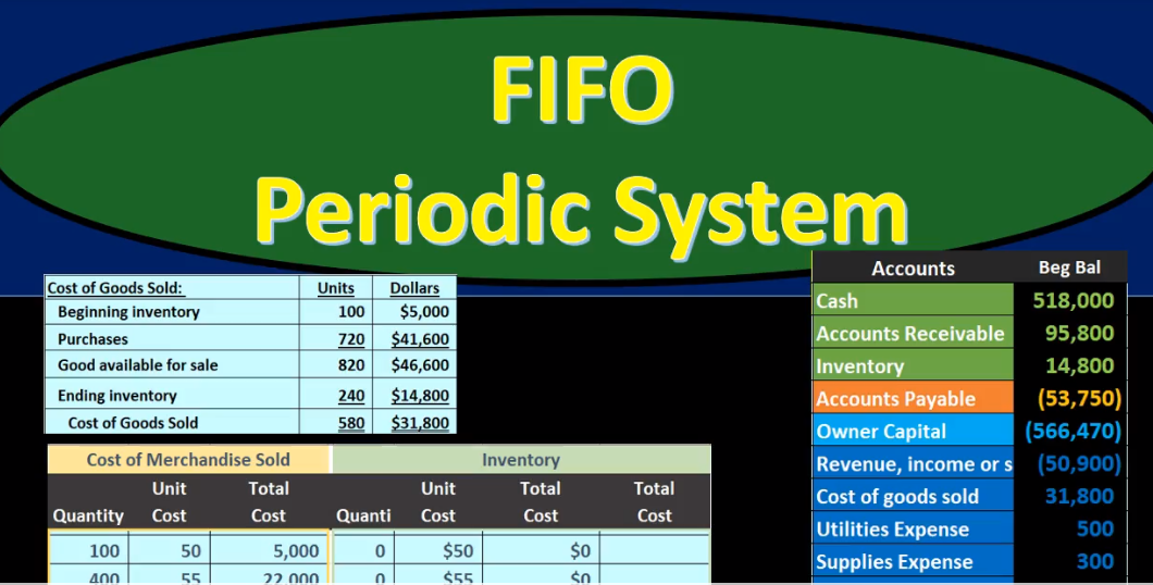
You do however, need to know what available goods available for sale is, or need to be able to interpret that subtotal because it is often it used in questions and in practice. So in our problem, the beginning inventory was $100, or 100 units at 50,000 $5,000. So we’re going to start with units 100 units. And then we purchased and this is the reason we have this purchases broke out separately 400 plus 120 plus 200, giving us 720. That’ll give us the available for sale 720 plus 100, or 820. That means that we had 820 units that went through the widget warehouse at some point in time, and therefore could have been sold at during this period this month. Then we’re going to do the physical count, we counted what’s still in the widget warehouse and there’s so 240 still there. So if there’s 240 still there and we could have sold 820 the difference then is 580 or cost of goods sold. Now note that it could have something else could have happened. We could have lost him we could have damaged Some damaged goods or what a spoil goods or whatever.
21:03
But we’re assuming that under the periodic system and that’s one of the faults of a periodic system that it’s so it’s sales that happened here this this number is due to a selling things. And the shrinkage of other things that could have happened, hopefully is in material. The perpetual system when we do the same calculation is primarily or one major purpose of it is not to record the inventory, but to detect that kind of shrinkage and problems with the inventory. Now, if if we knew exactly that these inventories were all purchased for the same amount, then we can just do an easy conversion and figure out what the dollar amount is. However, they’re not purchased for the same amount. This was 5055 6062. These are all the same widgets, but because purchased at different times, they cost different amounts. So that’s our problem here. So doing the conversion will get a little bit tricky. Let’s go through it same calculation Cost of Goods Sold calculation with dollars. We started with $5,000 worth, because we can do that conversion.
22:08
That’s where we started at the end of the last time period, then we had purchases of 720. And in dollars, we know exactly what we’re going to pay it was 20 to 7000 to 12,004. Even though these are different dollar amounts, we know exactly what they’re going to pay. It’s not an assumption. There’s no difference in either method, FIFO LIFO, average, perpetual periodic, we’re going to work out we bought 41,600 of purchases. So the goods available for sale then is 46,600 5000 plus 41. Six. That’s what we have here. That’s basically what we’ve been tracking on our worksheet. What we don’t have is the ending inventory in units. We know that I mean, in dollars, we know that units were 240, the units here 240. And those consist of these units, some of these units, so So 240 of these units here, the 100, the 400, the 120, and the 200 that we purchased throughout throughout this time period are still there. The question is, which one of them are still there? And how do we break out this number 46 600 between ending inventory and cost of goods sold. And that’s what we’ll do.
23:21
That’s where this cost flow assumption will come into play the lastin first out assumption. So, we have the lastin first out assumption. Now note you could kind of view this from either a indian indian ending inventory point of view or a cost of goods sold point of view, meaning you could say hey, ending inventories 240. And if I sold the last in was the first out I would have sold these ones first, the 200 and therefore figure out how much of them are still left, go back up here and try to save this 200 this 100 would be there and try to get up to this ending inventory of 200 40 or you can do what we’re going to do here, we’re going to say, There’s 580 that were sold according to the number of units. And therefore, we’re going to go into this column, the column, we haven’t used the entire time period, the cost of goods sold column, and figure out the cost of goods sold not for one single time period, but for the entire month, the month of March. So we’re gonna make our assumption here, here’s our layers that cost 5055 60 and 62. Here we have our cost flow worksheet. Again, we’ve got 100 units at 50, the 400, a 55, the 120 at 60 and the 262. We could take this we could look at that Indian inventory and try to decide how much is left we’re talking about a lastin first out system.
24:45
Therefore, these are the last ones we purchased at the bottom. Those would be the first out so we can take of what’s left and we can start saying okay, this hundred would still be there because those would be the last to go so up to 140 that are still there. that 100 would be there, and then see how much would be left at 140 of this layer would be left. Or we can think of it first as the cost of goods sold. What did we sell this is the new thing that we haven’t been dealing with with this entire problem. Until now the column we would be dealing with, on a perpetual basis at the point of sale under a perpetual system. But under a periodic system, we’re only going to be recording at the end of the time period. So we’ve got the cost of goods sold than 580, meaning we sold 580 units. So we could record over here which ones we sold, meaning under lastin. First out, the last ones been at the bottom, we’re going to count up from 200 up until we get to 580 and eliminate that what we had in inventory in this format. Note you might be thinking what’s a little backwards? Why would we be selling the last ones first, what kind of company would want to sell the last inventory first and the assumption Probably is not as accurate in terms of the actual flow of inventory, or at least the desired flow of inventory.
26:08
But because it’s just an assumption, we don’t know which inventory was sold, we’re not tracking them where they could have been could have taken any of the inventory. They’re all the same types of widgets. Therefore, we can make the argument that a lastin first out method is just as plausible as a first in first out method given the fact that we just don’t know. And so here we go, we’re going to say that the 200 here is going to be wiped out first. Those are the first units sold. So we’re going to say these are going to be gone at 6262 is pulling over, and that’s the 12,004 that’s part of the cost of goods sold part of the 580 units we sold here’s the dollar amount related to our 200 units of that 580. Then we’re gonna say that this 120 these are going to be wiped out as well, at $60. If we multiply that out, that’s the $7,200 of open sold Now we’re at 320, we need to get to 580. So we’re going to go into this 400. And pick out as many as we need to get there. We could do the math of 580 minus 120 minus 200 gives us 260. Or in other words, 260 plus 120 plus 200 gives us the goal of 580. Those are how many units we sold. So these 260 will be at $55. We multiply that out 260 times 55, we get the 14,300, the 12, four plus the 7002 plus the 14,300.

27:39
That is our cost of goods sold for the entire time period, the entire month, the month of March. Then we’re going to figure out what is left how much is still in Indian inventory. And so what we’re going to do there, it seems a little bit bad. It’s a little bit more difficult to think about this than the first in first out where we could just kind of compare Top to bottom, we can compare here we can say, well, this bottom layer is wiped out, I’m going to leave some space. And I’m going to put the entire four columns here. So of the four columns, the 200, what we did first, so this 200 right here, time minus the 200 means we have zero of those left at 62, those are gone. of the 120. Here’s the 121 20 minus 120 is zero, those are gone at 60. So these at 60, there’s none left. And then of the 400, before hundred and minus the 260 gives us 140 left, that will still be there. Those are at the 55 for 140 times 55 means we have ending inventory of 707,700. And then of the 100. Of course, those are all going to be brought down here. They haven’t been touched. And there’s the 50 There it is.
29:00
And so that’s going to be the effect of the lastin. First out, we might have this old layer on there forever, because if we never, we always have new layers, we never get to sell that old layer. And over time, this $50 will be quite low in comparison to what they actually cost at some at some point in the future. Now we can populate this information over here, we’re going to say Indian inventory. Well, if we add this up, we got the 5000 plus the 7700. Everything below this line we’re working with now 12,700. That’s going to be the ending inventory. We can now calculate cost of goods sold as either cost of goods available for sale 46,600 minus 12,700. Or take the same amount should be the same 12,004 plus 7002 plus 14,003. will give us that 33,900. Now we’ll do the adjusting entry.
29:55
That entry we haven’t been doing under the periodic system which we would see under a perpetual system reducing the inventory and recorded the related cost of goods sold at the point of sale under a perpetual system not being done until now until the end of the month. The end of march in this case, is a periodic system. So note that when we make a sale under a perpetual system, we record the first half of the journal entry, increasing the accounts receivable and increasing revenue debit accounts payable and credit revenue. What we do under a perpetual system that we don’t do under a periodic is at the point of sale record the decrease in inventory and related cost of goods sold. And in the periodic system, we’ll do that at the end of the process. We’re recording that second half, not for one transaction only however, but for the entire period the entire month, the month of March. We can see that of course the inventory now before that time period is overstated as is the will the cost of goods sold is understated. It’s at zero right now, until we make this adjustment.
30:59
So the adjustment will be inventory has a debit balance, we need to make it go down for all the sales we have made through the month of March. So we’re going to do the opposite thing to it a credit cost of goods sold is an expense account. And so we need to make it go up with for the expense of what we have consumed inventory in order to help us generate this revenue over the month of March. So we will debit Cost of Goods Sold debiting the expense crediting inventory. So this is going to be that journal entry that journal entry that again, we would see this form every time we make a sale under a periodic under a perpetual system every time we make a sale. However, under a periodic system, we only see it at the end of the time period, recording the cost of goods sold and the reduction in inventory for the entire month in accordance with the physical count. So that’s how we determined what the adjustment will be. It’s going to be coming from this cost of goods sold.
31:55
So once we posted, we’re gonna record the cost of goods sold and the reduction of inventory the reduction Bin Bin Tori bin should result in an Indian inventory of 12,700. You can see that we have currently 46,600, which is our goods available for sale, which we are now allocating between what is left in Indian inventory and what has been sold and is now in cost of goods sold the income statement account. So if we post this out, then we’re going to say Cost of Goods Sold started at zero, it’s going up by 33,900 to 33,900. Inventory started at 46,600, it’s going down by 33,900 to 12,700. That 12 seven matches what’s on our worksheet here, as does the 33 nine in cost of goods sold. If we look at the full transaction, then we can see that our inventory is much lower than before this end period adjustment and our cost of goods sold is much higher.

33:00
Which brings net income down substantially. So net income was 40,001 80. Before this went down by 33,900 to 6002 80. So until we record this adjustment under a periodic system, we can’t rely on our net income number, it’s going to be completely wrong because the cost of goods sold is the biggest expense. Typically, for a merchandising company, our assets will be way overstated as well, because they will not be recording the inventory being decreased as sales happen until the end of the time period. So it will be a good system at the end of the time period once this adjustment has been made. If we look at all the components, here, we can see our matching of the cost of goods equation, we’ve got the ending inventory here, the ending inventory on our worksheet, and the ending inventory on the trial balance. We have the cost of goods sold and the cost of goods sold calculation, the cost of goods sold would be the same number here. 12,004 plus seven thousand two plus 14,003 adds up to 33,900. And we see it here in the cost of goods sold on the trial balance.