
In this presentation we will discuss the weighted average inventory method using a periodic system. The weighted average method as opposed to a first in first out or last In First Out method, the periodic system as opposed to a perpetual system. We want to keep the other systems in mind as we work through this comparing and contrasting. We’re going to be working with this worksheet entering this information here. It’s important to note that this worksheet is a worksheet that can typically be used with any of these inventory flow type problems of which there are many. We have first out last in first out the average method. And then we have a perpetual and periodic system which can be used with any of those methods. It’s also possible for questions to ask for just one component such as cost of goods sold or Indian inventory, and therefore it can seem like there’s more types of problems that we can have in that format as well. If we set up everything in a standard way, even if that weighs a little bit longer for some types of problems, it may be easier because we can just memorize that one format to set things up, this would be a format to do that.
01:09
This would be breaking up the information into three components purchases, cost of merchandise sold and inventory or ending inventory. Within those three components, we’re going to have the quantity, the unit cost, and then the total cost in each of these three sections. And then we’ll enter the data through this worksheet as we go starting this time with the beginning inventory. So this is where we started at the beginning of the month, in this case, the month of March, we’re going to say the beginning inventory is 100 units, costing $50 100 times 50. Being 5000. We’re going to put that same 5000 out to the total column, just to give an indication as we go through this worksheet of what the total is in its own distinct column out in the total section. So there we have that 5000 units. That’s where we start. If we look Add our trial balance it will be an order assets, liabilities, equity, revenue and expenses, debits, non bracketed or positive numbers, credits, bracketed or negative numbers, the debits minus the credits equaling this zero.

02:14
We have net loss in this case, meaning revenue of zero minus these expenses five, three and 9009 20 given us a loss of 10,007 20. We’re focusing here of course, this time being the inventory on inventory, this 5000 matching what we just put into our worksheet, that is our beginning balance. That’s where we start. Next we will have a purchase of 400 units at $55. We’re going to put that into our worksheet in the purchasing section. Remember that the purchases will not differ no matter what method we will be making, whether that’s FIFO LIFO, average, perpetual or periodic it will be what it is, in March. It was 400 units that we purchased at $55. Notice the rising prices from 50 to 55. For the inventory units, we are purchasing same units costs going up, that’s going to be the standard assumption that will happen, we want to just remember going one way as if cost increase would be the norm. And then if it goes the other way, then we can kind of just reverse some of the effects that would happen. So in other words, as costs rise, what’s going to be the effect on ending inventory and cost of goods sold under the three methods LIFO, FIFO, and average, and then reverse the effects, obviously, when costs then fall, so we’re gonna have the 400 times 255, that’ll be the 22,000.
03:38
Then we’re going to do our average calculation. Now it’s possible since we’re doing a periodic system to just do all of the purchases and then calculate the average at the end. But we’re going to calculate the average as we go to get practice calculating the average it can be something that people find a little bit more confusing, because of the weighted average that we will be using. So What we’re going to do is we’re going to calculate our average by putting the calculation all under this line under this date line, again, moving this amount down. So there’s our hundred units at 50, or 5000, then we’re going to move this column over, and there’s our 400 units at 55. So we started at 100 units at 50, we got 400 units at 55. What we want to do now is create the average. Now I’m going to show the wrong way to do this first of all, and then we’ll calculate the weighted average. So the normal average of just the two prices would be 50 plus 55. Those two numbers divided by two
04:38
would give us an amount right in the middle of them at 5250, which seems reasonable 50 to 50. Seems reasonable. However, it’s not exactly right, because there’s a lot more of the 55 units 400 than the 50 units 100 and therefore the weighted average taking that into account would be closer to the 55 then to the 50 So that’s the mistake, we just have to kind of avoid, how are we going to do this, we’re going to take the total here, the total dollar spent and the total units, and then divide those out. So it can look look a little bit confusing on the worksheet because we’re first going to calculate or sum up the units 104 hundred, we’re not going to sum up the unit cost, that doesn’t really make any sense. Because it’s the unit cost, we can sum up the total here 5020 2000 for 27,000, and then take this 27,000 divided by 500. So now we’re simply taking the 27,000 divided by 500. And that gives us the 54 which is closer to this number, that’s the weighted at the 400 units. So we get 54 as our total. If we pull that out to the outer column, then the 27,000 what is what should be on our financial statements in Ending Inventory and our trial balance. We’re going to record the journal entry here. Now here’s going to be our new thing that happened, we purchased another 400 units. For 22. We’re going to adjust inventory inventory has a debit balance, we’re going to make it to go up by doing the same thing to it another debit of 22,000 then the other side’s not decreasing cash but increasing the liability accounts payable.
06:24
Therefore we will increase accounts payable by the 22,000. posting this out then we have the inventory inventories up here it’s 35,000 it’s going to go up by the 22,000 to 27,000. Then we have the accounts payable, accounts payable 12,001 50 going up by 22,000 to 34,001 50. Note once again, this transaction is going to be the same no matter what method we are using. If we see everything here we’re going to say that we’re still in balance, no effect on net income the purchase of inventory was not expensed at At the time of purchase it will be expensed but not till it’s used in order to generate revenue in accordance with the matching principle that will be when cost when we sell it in the form of cost of goods sold. However, under a periodic system, we’re not going to get around to recording that cost of goods sold until the end of the time period until we do a physical count the end of the month, the end of March in this case, next transaction, we’re going to say that there’s a sale of 420 units at $85. Now if we were using a perpetual inventory system, we would have to record the reduction of inventory and the cost of goods sold along with this sale into our worksheet.

07:40
We’re not looking at the worksheet here because we’re in a periodic system, and we’re not going to record that component until the end of the period with a physical count. What we will record is just the journal entry just to demonstrate this journal entry the sales journal entry, which will be the same under the two methods a periodic and perpetual the second time He’s being the difference. So remember that if we make a sale on a merchandising company we typically assume that it’s going to be a perpetual system. And we often break out that journal entry when considering it and thinking about it into two journal entries meaning we have the sale side and then we have the the inventory or cost of goods sold side of the journal entry. The sales side we can think of as similar as if we were a merchandising company and we can just eliminate the inventory and say, hey, what would happen if we had a sale or did services and got paid or on account meaning we got an accounts receivable what would be the journal entry? Cash is not affected. Accounts Receivable has a debit balance, we got more of it, people owe us money. Therefore accounts receivable will go up with another debit.
08:47
So we’re going to debit accounts receivable and then we’re going to credit something and something will be revenue. That revenue for a service company might be fees earned, or it might be revenue or income and it could be called sales for a merchandising company. But it’s all just a revenue account. So it’s going to go up in the credit direction. This is kind of our normal journal entry that we see whenever we make a sale, whether it be merchandise or a service type business accounts payable going up, revenue going up. Then we have the second component that we typically think of when we make a sale as a merchandiser, meaning we sold merchandise inventory should be going down, and the related Cost of Goods Sold should be going up. We’re not going to record this under a periodic system. That’s the difference between a periodic system and perpetual system, we’re only going to record the decrease in inventory and related Cost of Goods Sold expense at the point at the end of the period, the end of the month, in this case, the end of March, after we do a physical count, why why would we do that? Why would we not decrease the inventory? We know the inventory went down, and it’s probably just the sophistication of the system.
09:57
If we if we’re have a clerk or somebody In recording the sales, it’s easy to know what the sales price is. But this sales price has nothing to do with the cost of goods sold. Or in other words, the cost of goods sold might have been used to make that sales price. But this there’s no direct relationship between these two things. The sales price is no one when we make the sale. So 420 times 85. That’s the 35,700. That’s what we want to focus on collecting the revenue and making the sale at the point of sale. We don’t want to spend all of our time training people how to record the the cost of goods sold or inventory, if they have to do it manually, because that could take some time, especially if there’s multiple products that we are selling. If however, it’s an electronic scanner system that does it at that point in time without us even needing to know what the cost is, then that makes it a lot more doable to do a perpetual system, which would be better from an accounting standpoint. If we don’t have that sophistication, we may Using a periodic system, which will simplify the process, but we know that it won’t be entirely accurate until the end of the time period.
11:09
So if we post this out, then accounts receivable, debit balance, we’re posting this 35,000 to it, going from 44,900 up by 35,700 to 80,600, then the revenue is going up from zero, we’re posting this revenue up from zero by 35,700 to 35,700. If we look at our full transaction, we’re back in balance, net income is going up, drastically went up a lot and went up by 35,700. So 35,700 minus these expenses is 24,009 80. So that’s going to be our net income note, it’s really not exactly correct. Now, of course, because we haven’t recorded the cost of goods sold, and that’s going to be a substantial expense that we haven’t recorded. We haven’t recorded the decrease in inventory. So our assets are overstated we will do so at the end of the time period, the end of the month, the end of March.
12:07
Next we have on 318 purchased 120 units at $60 per unit. So once again we’ll be in the purchases column, this will be the same as in any method first in first out last In First Out average perpetual periodic, these purchases are what they are, this is what we will actually pay for the inventory, we’re going to have the 120 units at $60. Note the rising prices from 50 to 55 to 60. That’s not because the units got better. That’s not because we’re buying better widgets or better inventory, the price is just going up. And that’s going to be the standard prices increasing the standard for these types of problems to standard for practice, as well due to inflation. If nothing else, the 120 times the 60 will give us the 7200. Now we’re going to calculate the average once again, remember that if we’re doing a periodic system, we could calculate the average basically At the end and sum of all of them, but I want to calculate the average each time we make a new step. Because this is the most complex component. Typically, what we’re going to do is draw a line here, we’re going to bring this amount down. So this is what we had before, we have 500 units at $54. That’s 27,000, then we’re going to pull over the new information. Here’s the new information.
13:23
What we are not going to do when calculating the average, what you want to avoid, be careful of, is to just take the amounts the 54 plus 260, the 54 being the old average plus what our new inventory costs, and taking that in dividing it by two. What’s the problem with that it looks like a reasonable number. But it’s not taking into account the weighted average. It’s not taking into account that we have 500 units at 54 and only 120 at 60. And therefore, this number should not be right in the middle but leaning towards the 54. So instead, what we’re going to do is Come up the total units, we have the 500 and the 120, then sum up the total dollar amount that we paid for those units 34,200. And then we’ll do the division problem, that division problem being the 34 200 divided by the 620 units, given us a number of 5516. Note, it’s not going to round specifically to the penny, that’s okay, that happens in practice, we’re going to round it to the penny because we’re talking about dollars and cents here. So we’re going to say that, calculate that that’s that number here is going to be this number divided by this number with a total dollar amount divided by the quantity. So that’s going to give us the 34,200 that we want to get to on our trial balance. Now in our financial statements, we’re going to do that record in the journal entry. The journal entry will be the same under any method FIFO or LIFO average because it is a purchase. That’s not the side that differs. The side that’s different is when we make the sale. So we’re going to say that inventory has a debit balance, we need to make it to go up. So we’re going to do the same thing to it, another debit. So here’s the debit to inventory, the other side’s not going to be paid with cash, we’re going to increase the liability. So the liability has a credit balance, we’re going to increase accounts payable, therefore by a credit of 7200. posting this out, then we have the inventory in the journal entry.
15:24
The inventory up here in the assets we started with 27,000, it’s going to go up by 7200 to 34,200. Then we have the accounts payable, we have the accounts payable here, it’s at 34,001 50, we’re going to increase it in the credit direction 7200 to 41,003 50. So there’s going to be our transaction this 34,200 matches what we just calculated on our worksheet that 34,200 the inventory worksheet supporting the inventory amount reported on the trial balance Or the balance sheet, here’s going to be the full transaction, we still have the 34,200. We’re back in balance indicated by the green zeros, no effect on net income no effect on these accounts, the revenue or expense accounts, we will be affecting the revenue expense accounts by the inventory that we purchased not at the point of purchase, but at the time we sell the inventory in the form of cost of goods sold. However, under the periodic system, we won’t be recording that until the end of the period when we do the physical count. We’re gonna do another purchase here purchased 200 units at $62. So we are going to be in the purchases column once again, the $200 per 200 unit purchase at $62.
16:42
Note the rising prices going from 50 to 55 to 60 to 62, same units, unit costs going up because of If nothing else, inflation, that will be the norm. You want to think that it can go down, but you probably want to think the norm will be increasing prices and in reverse your thought process for it to go down that 200 times 262 gives us 12,400, we’re going to calculate our average now. And we could do this at the end of the time period under periodic system for the average method, we’re going to do it as we go, this being the key component to the average system, calculating that average cost. To do so we’re going to draw a line under there last dateline. And we’re going to be putting this new information here taking this to 620 down, just copying that down, and then we’re going to pull over our new information. And once again, we’re going to say what not to do, which is a common common error in calculating this and that’s going to be taking the 55.16 plus the 62, or the two prices and just dividing by two.

17:47
That’s an average but it’s not the weighted average because it’s right in the middle of those two costs and it should be leaning towards the 620. It been weighted higher it having more inventory in it. So What we’re going to do instead is we’ll sum up the 620 and the 200 to get the 200, the 820, then we’ll have the 34,200 and the $12,400 amount to get to the 46 600. And then we can do our average, we’re going to take the total dollar amount, the 46 600 divided by the 820 units, giving us a average of 5683. rounding up not worrying about the fact that we have all these decimals, we’re going to use the rounding to the pennies, talking dollars and cents. So that’s going to give us the 5683. That’s going to be this number divided by this number. There’s the total that we are going to be reporting on the financial statements. We will now record the journal entry for that new purchase the purchase of the 12,400 remember that the journal entry will be the same under LIFO FIFO, average periodic perpetual, all of them this is not an estimate.
18:56
We’re going to say that the inventory started at the debit balance We’re going to increase it, we bought more inventory with a debit of that 12,400. We’re going to credit not cash, but the liability of accounts payable, increasing the accounts payable. posting this out, we have the inventory here go into the inventory, they’re starting at 34,200 increasing by 12,400. Go into a total of 46,600. Here’s the accounts payable there, it’s going to be posted here we’ve got a credit balance starting at 41,003 50, increasing 12,400 to 53,750, noting that the inventory that we end up with is supported by our inventory worksheet. Now we’re going to do the inventory count at the end of the time period. This is what we’re going to do in a periodic system in order to record the cost of goods sold for the entire period what we have not been doing for the entire period and record the related reduction in inventory, something we haven’t done so you’ll note that as we go in our worksheet we’ve just been doing purchase And we’ve been increasing and increasing with purchases, not recording the decrease in the inventory for the sales.
20:07
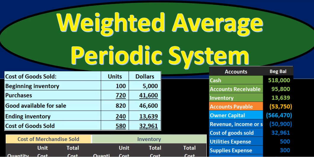
And we’re going to do that at the end of the time period due to and with the help of a physical count and the cost of goods sold calculation, Cost of Goods Sold calculation a mandatory calculation something we really have to know both in terms of units and in terms of dollars. The format will look like this beginning inventory plus purchases gives us goods available for sale or mt available for sale, minus the ending inventory will give us cost of goods sold. That’s going to be our calculation. Now note that a multiple choice question might ask you for any component just give you three. One unknown for this formula, they might give you the beginning inventory as the unknown, for example, or the purchases as the unknown. Now you could write this formula as beginning inventory plus purchases skip the subtotal, beginning inventory plus purchases minus ending inventory. Worry equals cost of goods sold, and write it out as an algebraic equation. given any of these unknowns, then as long as we only have one, we would then be able to find out any of these amounts. So keep that in mind. You don’t want to remember multiple different equations to figure out for example, purchases, or beginning inventory, you want to remember one equation cost the goods sold, they can answer any of those types of questions. Or you do need to know the subtotal. However, by name, even if you don’t use it in the equation, if you pull it out for an equation, because some problems will refer to it as well as in practice. We’re going to do this calculation first for the units and then we’ll do the same calculation in terms of dollars. We started off with 100 units. That’s what we began with.
21:46
We purchased 720 units 400 plus 120, plus the 200 in the purchases section. That gives us 820 available. That doesn’t mean we had 820 at any given time in our warehouse. But within the widget warehouse, we had 120 go through it, meaning we started with 100. We purchased 720. We may have sold items throughout here, we don’t know what we sold. But we know what we purchase and therefore had available for sale, hence the name goods available for sale. And that’s 820. Then we’re going to do the physical count. So we’re going to say there’s 240 widgets left and then widget warehouse. So there’s 240 left. So we had 820, we could have sold 240 are still there, given our physical count, then the difference between the two is 580. That’s what we sold in terms of the widgets. It is possible that we had shrinkage or thefts or spoilage or something as well, which is why the perpetual system would be nice to use, because it can verify or better verify that type of problem. But our assumption is sold and the assumption is that the shrinkage of any kind breakage or theft is In material in in relation to it, and therefore, we’re going to record this entire amount to cost of goods sold.
23:06
So note what we did here, we just basically said, Hey, this is the amount we had available, and then allocated it out between either what’s still left in Indian inventory and what has been sold, we’re gonna do that same thing with dollars, it would be a very easy conversion if the dollar amount were the same throughout the entire period. But very often, it is not even though we’re talking about the same widgets, we’re not buying different types of things. It’s all the same, but the dollar amounts are increasing. So that makes it a little bit difficult. If we see this, then we’re going to say, well, we started with $5,000. That’s our beginning balance, we know that we purchased 720. And we purchased them for 41,600. We can’t convert from 720 to 41. Six easily because of the different dollar amounts. But we know what we purchased we can just look at the CIO and say, Hey, we, we increase inventory. That’s how much we’re gonna pay. It’s not an estimate. This is what we’re going to pay 22 thousand plus 7000 t plus 12,004. That’s a given. That’s not an estimate.
24:05
And so if we add those two up, we’re at 46,600. That’s where we start. Now we’re going to allocate that out between ending inventory and cost of goods sold. However, we know that there’s 240 units that we’re still in ending inventory. But now we have to figure out our conversion here because we need to know which of those units we purchased some for 50, some for 55, some for 60, some for 62. That’s what we’ll do now on the average method. And the average method because we’ve been calculating it as we go is nice and easy right now, we’re just going to say, Well, yeah, some of them cost 5055 50 to 60, whatever, but they all cost around about an average if we average them all out a weighted average of $56 and 63 cents. So we’re going to say whatever we sold, in this case, 580 units, those 580 we sold for this 5683 about if we multiply 580 times 5683, we get 32,960 93. And that’s our cost of goods sold. This is the cost of goods sold, we haven’t been recording the entire time period. It’s the cost of goods sold that we would record every time we make a sale under a perpetual system, the cost of goods sold we are now recording for all sales happening during the time period, in our case, the month, the month of February, March, month of March.

25:23
So we have 820 units that we had before minus the eight the 580 means we still have left 240 so we did this allocation of the 820 units 580 have been sold and 240 are still left. They are at 5683. If we multiply 240 times 256 83, we get 13,006 3902. So now we can fill out the rest of this form we can say okay, the ending inventory is 13,000 969 3639 don’t have to. And we could subtract this out then. And notice we did take off the round in here. So here we have the pennies. Here we remove the pennies, it’s just rounding. So if we take off the 46 600 minus 13 639, we get the 32 961, which is also matching this amount 30 to 960. Rounding 961. So that’s how that ties out, we’re going to do our final journal entry. Now, this would be the journal entry that we would see under a perpetual system, every time we record a sale, or similar one, at least one that would be reducing inventory and recording cost of goods sold. But under a periodic system, as we are doing now, we will only see one time, at the end of the period, whatever period that may be, for our case, the month, the month of March.
26:46
So we’re going to record the reduction of inventory for the entire time period. Inventory has a debit balance, we’re going to make it go down by doing the opposite thing a credit and the related cost of goods sold. Cost of Goods Sold is an expense. It’s going to go up In the debit direction, bringing net income down. So here’s the cost of goods sold. And there’s the inventory. So once again, this is the journal entry, we would see each time under a periodic system. As we record sales, it’s going to be the second half of the sales transaction. But under a perpetual under a periodic under a, that would be the case under a perpetual system. But under a periodic system, we’re only going to record it for the entire sales all sales made during the period at the end. So if we record this, here’s cost of goods sold, here’s cost of goods sold here, it’s going to go from zero way up by 32,009 61 to 32,009 61. Here’s inventory, here’s inventory, it’s at 46,600. It’s going to go way down by 32,009 61 to 13,006 39. This number now matching the 13,000 in Indian inventory, this number now matching our cost of goods sold calculation. So notes Before we did this transaction, our net income was way too high.

28:04
And now it’s way lower. So that’s going to be the case for the periodic system, our net income cannot be trusted. Until we do this transaction, the cost of goods sold been huge for a merchandising company typically, also our assets will be way overstated, until we do this end of period adjustment because once again, the inventory is typically a fairly large asset. And it’s not being reduced as we make the sales. So we got to wait till the end of the period to have an accurate number there. If we look at the comparisons, here’s our calculation. Here’s our worksheet. Here’s our trial balance, we can see that we have the ending inventory here we have the ending inventory on the trial balance, which would be on the financial statement. We have the ending inventory on our worksheet. We have the cost of goods sold here on the cost of goods sold calculation costs get sold on our merchandise, Cost of Goods Sold worksheet, and then we have The cost of goods sold here on our trial balance as well which would also be on the income statement.